Teaching a Computer to Design Waveguides
Designing a good constant-directivity waveguide is not a one-afternoon problem. The geometry — throat profile, flare shape, mouth size, wall angle transitions, cross-section morphing — couples into the far-field polar pattern in ways that are non-linear, frequency-dependent, and deeply sensitive to small changes. For decades the standard workflow has been: intuition, prototype, measure, iterate. Manual. Slow. Expensive.
I built a tool to automate that loop. It orchestrates three separate programs — ATH4, GMSH, and ABEC3 — drives them through hundreds of parameterised simulations, scores each result against a multi-term acoustic objective, and uses Bayesian optimisation to find the best geometry without a human in the loop. This is a technical write-up of how the whole system works.
ATH4 generates waveguide geometry from the Oblate Spheroidal Source Equation (OSSE). GMSH meshes the surfaces. ABEC3 solves the BEM problem. The ATH4 Tool drives all three automatically, scores the acoustic result, and uses Bayesian optimisation (Optuna / TPE + CMA-ES) to search the parameter space.
Six modules handle different parts of the workflow: batch setup, results browsing, manual comparison, parameter sweeps, Bayesian optimisation, and IB-vs-box calibration (Score Lab).
A typical optimisation run produces a ranked database of hundreds of designs in a few hours — on hardware that would take weeks with manual iteration.
The Geometry Engine: ATH4 and the OSSE
Before anything can be simulated, the waveguide geometry has to exist. ATH4 is a parametric geometry engine for constant-directivity horns and waveguides. It takes a small set of design parameters and produces a fully-meshed 3D surface geometry ready for BEM simulation. Understanding what it does — and why — requires a detour into the mathematics it is built on.
Oblate Spheroidal Coordinates
The standard Cartesian or spherical coordinate system is a poor fit for describing waveguide profiles. Spherical wavefronts diverge too rapidly; plane waves do not flare at all. The Oblate Spheroidal (OS) coordinate system sits between these extremes and turns out to match the actual acoustic behaviour inside a flaring horn much more closely.
In oblate spheroidal coordinates (μ, ν, φ), surfaces of constant μ are oblate spheroids — flattened ellipsoids whose focal ring lies in the throat plane. The defining transformation from Cartesian coordinates is:
y = c ⋅ cosh(μ) ⋅ cos(ν) ⋅ sin(φ)
z = c ⋅ sinh(μ) ⋅ sin(ν)
Here c is the semi-focal length, set by the throat geometry. The μ-coordinate tracks depth along the horn axis; ν is the angular coordinate that determines coverage angle. Constant-μ surfaces are the natural wavefronts for a source radiating into this coordinate system — they start as a flat disc near the throat and progressively inflate toward a hemisphere far from the source.
The Source Equation
The Helmholtz equation separates cleanly in oblate spheroidal coordinates. The resulting equation for the μ-dependent part of the pressure field is the Oblate Spheroidal Source Equation (OSSE). Its solutions describe how the wave amplitude and phase evolve along a waveguide whose walls are aligned with constant-ν surfaces — i.e., walls that subtend a fixed angle θ from the axis at every depth:
This is the constant-directivity condition. If the waveguide walls track a constant-ν surface, the local coverage half-angle θ is preserved as the wave propagates from throat to mouth — at least in the limit of an ideal, continuously-flaring, infinite-resolution geometry. Real waveguides deviate from this ideal due to diffraction at the mouth, finite aperture effects, and driver non-idealities, which is precisely why simulation matters rather than just trusting the OSSE solution directly.
OSSE gives you the right shape to start from. BEM simulation tells you how far reality deviates from it — and Bayesian optimisation finds where to nudge it back.
ATH4: From Equation to Geometry
ATH4 implements the OSSE-based profile calculation and extends it in two important directions: azimuth-dependent coverage for asymmetric patterns, and cross-section morphing from the circular throat to an arbitrary target mouth shape.
The geometry is controlled by a small set of parameters in a plain-text configuration file. The key ones:
| Parameter | What it controls |
|---|---|
Coverage.Angle |
Target coverage half-angle as a function of azimuth p. Can be a full trigonometric expression, allowing different horizontal and vertical coverage in one geometry — e.g. 90° H × 60° V. |
Length |
Axial depth of the waveguide from throat to mouth plane, in mm. |
Term.s |
Radial terminal shape factor — controls how the wall profile curves at the mouth exit. Can also be azimuth-dependent to tune the mouth shape independently of coverage. |
Term.n |
Transition exponent. Low values give a soft, gradual flare; high values give a sharper wall angle transition closer to the mouth. |
Term.q |
Profile quality factor — how closely the generated wall follows the ideal OSSE surface (values near 1.0 are most faithful). |
Morph.Rate |
Controls how quickly the cross-section transitions from circular throat to rectangular target mouth along the axial direction. |
Morph.CornerRadius |
Rounding radius at the rectangular mouth corners, in mm. Affects both aesthetics and diffraction at the mouth edge. |
Throat.Diameter |
Compression driver exit diameter — fixed for a given driver, typically 25–50 mm for 1″ and 2″ devices. |
ATH4 outputs two things: the meshed surface geometry (triangulated panels, passed directly to GMSH for refinement) and an ABEC3 project file with the source configuration and simulation settings already populated. The Python tool then takes it from there.
The Toolchain: Three Programs, One Pipeline
No single program handles the whole job. ATH4, GMSH, and ABEC3 each do one thing well; the ATH4 Tool orchestrates all three from a single interface so that a trial that previously required manual handoffs between applications now runs unattended.
For each trial, the Python tool fills in the {VAR_X} placeholders in the template with the current parameter values, writes the resulting configuration to a numbered simulation directory, launches ATH4, waits for it to finish, then launches ABEC3 on the generated project, and harvests the output polar data. Geometry sanity checks (maximum cabinet width and height, mesh size limits) are evaluated before the simulation runs and prune invalid trials immediately without wasting compute time.
The ABEC3 simulation produces a complex-valued far-field pressure spectrum at 19 angles from 0° to 90° in the horizontal plane. That output file is parsed, fed into the scoring function, and the result is returned to the optimiser. The whole pipeline — from parameter proposal to score — runs in roughly 30 seconds per trial on modest hardware.

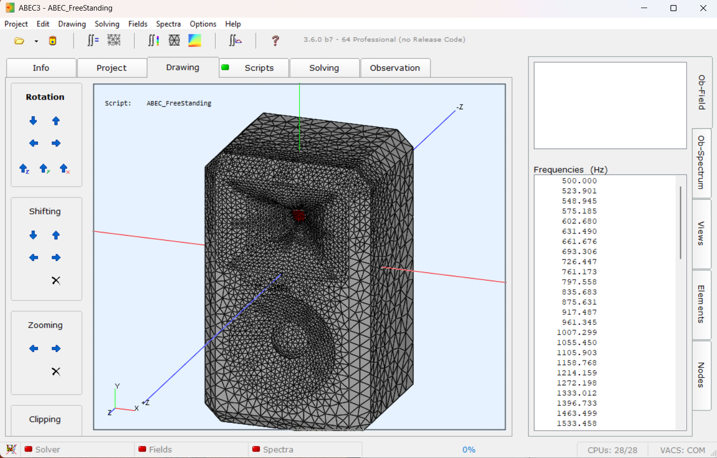
The Simulation Engine: Boundary Element Method
Every simulation in the pipeline is a BEM (Boundary Element Method) acoustic solve. Unlike FEM, which discretises the entire fluid volume, BEM only meshes the surfaces of the geometry and solves the Helmholtz integral equation on those surfaces. For exterior radiation problems — a waveguide radiating into free space — this is a significant advantage: there is no need to mesh and truncate a surrounding air volume. The radiation condition is satisfied analytically.
The Helmholtz equation in the exterior domain:
is recast as a surface integral using Green's theorem. The pressure at any exterior point can be expressed entirely in terms of pressure and normal velocity on the surface boundary Γ. Discretising Γ into N elements yields a dense N × N complex linear system assembled and solved at each frequency point. The solver is ABEC3 by RDTeam, a well-established commercial BEM code specifically built for loudspeaker acoustics.
The polar pattern is computed at 19 observation angles from 0° to 90° in 5° steps (horizontal plane), across 30–40 log-spaced frequency points from 500 Hz to 16 kHz. That gives 570–760 complex pressure values per simulation — the raw material the scoring function works with.
The Tool's Interface: Six Modules
The Python application is structured around six functional modules, each accessible from the sidebar. The first four are detailed below; the Optimisation and Score Lab modules are covered in their own dedicated sections that follow, since they require the scoring and search concepts to be established first.
Brute-force sequential simulation runs — every parameter combination in order. Useful for small grids, single-design verification, and sanity checks before committing to an optimisation.
Browse all simulations in a batch folder. Sonogram, polar waterfall, BW/DI curves, and parameter readout for any selected design. Re-run any design as IB or full-box from here.
Overlay BW and DI curves from multiple selected designs on one plot. Manual side-by-side comparison without leaving the tool.
Systematic single-parameter sweep across a defined range. Useful for understanding sensitivity: how does score or BW change as Term.n goes from 2 to 7?
Bayesian optimisation with TPE and CMA-ES. Persistent SQLite database, warm restart, live score history chart, and ETA tracking.
Takes top-N designs from an optimisation run, runs full-box BEM simulations on each, and computes Spearman rank correlation between IB and box rankings to validate and calibrate the scoring formula.
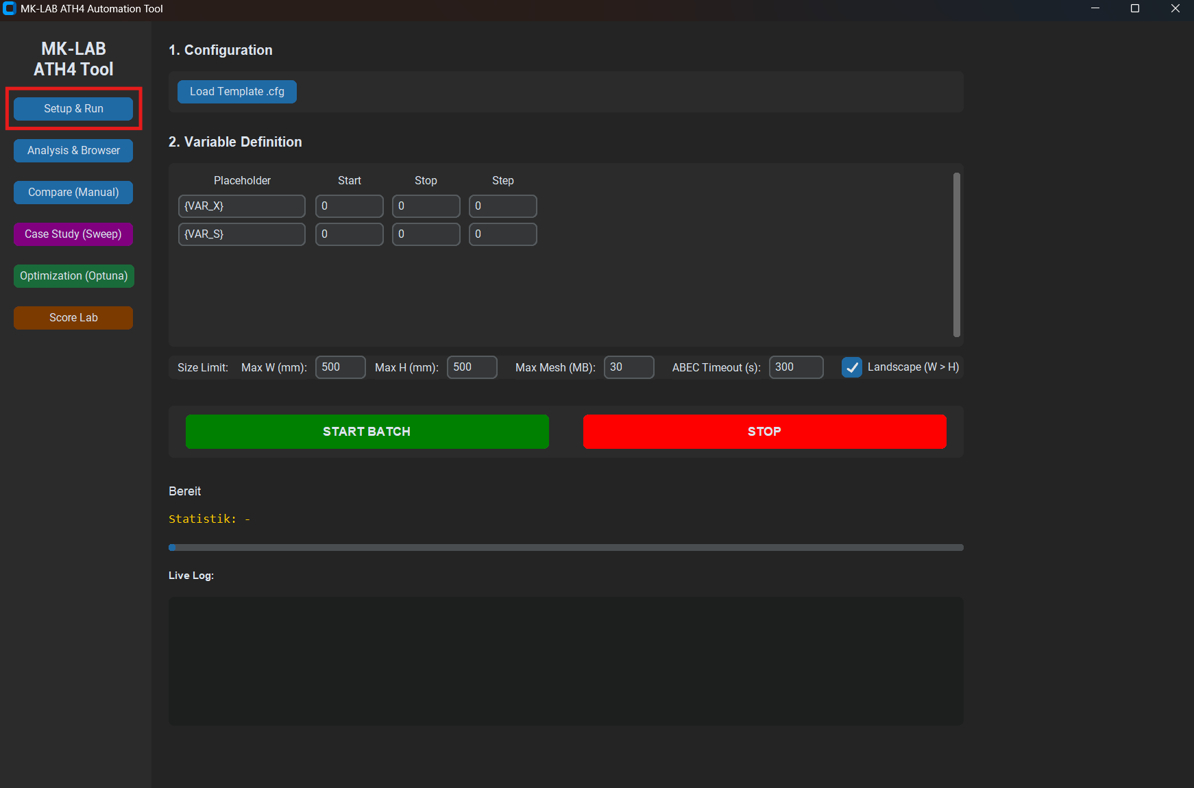
Setup & Run
The Setup tab runs a brute-force sequential batch: every parameter combination in the declared grid, in order, one after the other. It is not the right tool for exploring a large design space — that is what the Optimisation tab is for. But it earns its place for small grids (e.g. sweeping two or three values of a single parameter), for single-design verification runs, and for sanity-checking a new template before handing it to the optimiser.
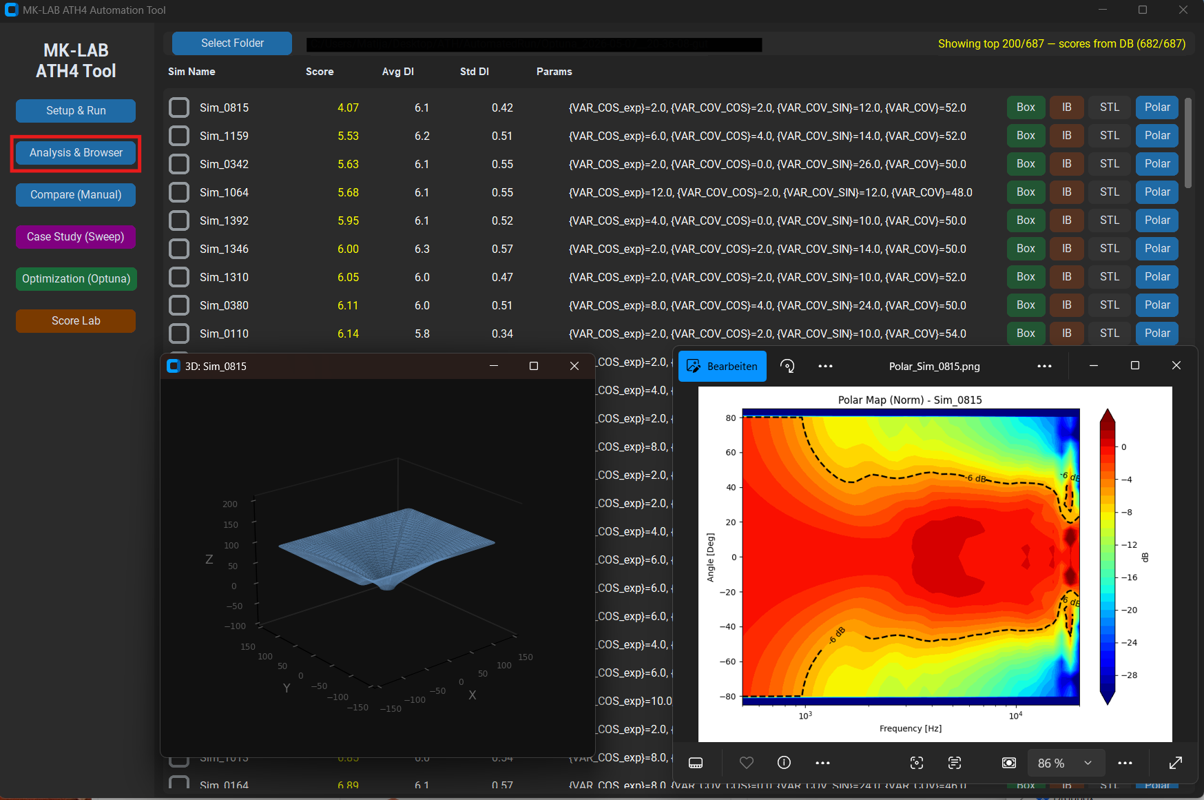
Analysis & Browser
After a batch finishes — or while it is still running — the Analysis tab provides a complete picture of every simulation in the output folder. Selecting any design from the list immediately renders its polar sonogram (SPL vs. frequency vs. angle), BW curve, DI curve, and the key T/S-style parameters extracted from the config. From the same panel, a design can be re-simulated in infinite-baffle or full-box mode with a single click, generating a new result in a paired subfolder for direct comparison.
Case Study: Single-Parameter Sweep
The Case Study tab runs a systematic sweep across one parameter while holding all others fixed. This is the diagnostic tool: when a design scores well but has a suspicious feature in the BW curve, sweeping Term.n or Morph.Rate across its full range while watching the resulting curves immediately shows whether the feature is sensitive to that parameter — and in which direction it needs to move.
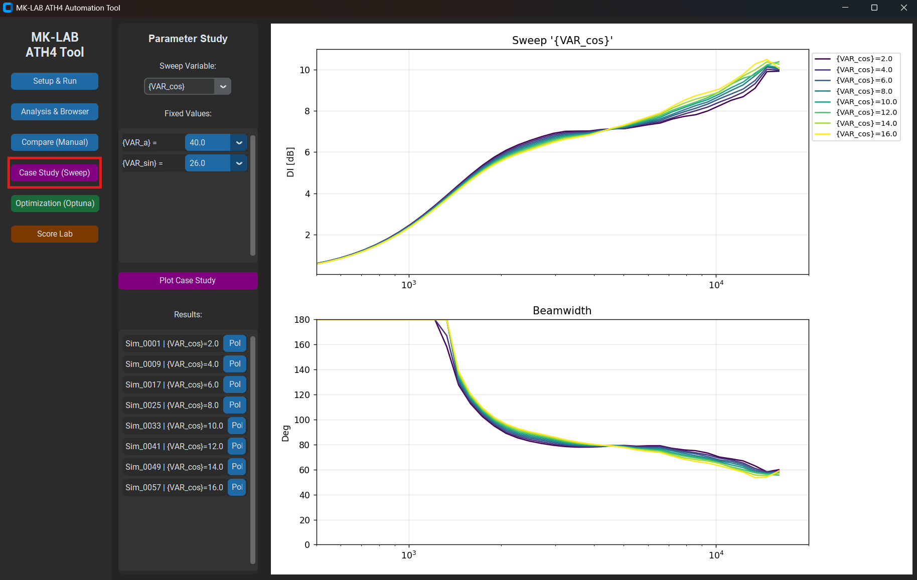
Term.n from 2 to 7 in 0.5 steps. Each curve is a full BEM solve. The overlay makes the sensitivity immediately visible — in this case, the mid-frequency BW narrows significantly above n = 5.
Compare
The Compare tab is the manual side-by-side view. Select any set of designs from a batch folder, click Compare, and the BW and DI curves are overlaid on a single plot. No further analysis — just a clean overlay for direct visual inspection of two or three candidates before deciding which to take forward into the optimisation or physical prototyping.
The Parameter Space
A waveguide geometry is described by the ATH4 parameters listed above. In the optimisation template, each free variable is declared with its bounds and step size using the syntax {VAR_NAME:min:max:step}. A step of zero means continuous (no grid). The constraints are also declared inline as comment lines — the tool parses them and evaluates them before each simulation, pruning invalid trials immediately.
A typical optimisation run has 10–14 free variables. The parameter space is a compact hyperrectangle in that many dimensions; the optimiser's job is to find the region that produces the best acoustic result.
Every additional dimension makes the search space exponentially larger. The tool keeps the count deliberately low — 10–14 active dimensions — so that a few hundred trials are sufficient for meaningful convergence rather than just scratching the surface of the space.
The Objective Function
This is the core of the system and the part that takes the most judgment to get right.
The raw outputs of each BEM solve are far-field complex pressures P(f, θ). From these I derive two secondary curves:
Beamwidth (BW)
The −6 dB full-angle beamwidth at each frequency: the angle between the two points where SPL has dropped 6 dB relative to on-axis. A constant-directivity design produces a flat BW curve across its operating band.
Directivity Index (DI)
How much more acoustic power the waveguide radiates on-axis relative to an omnidirectional source of equal total radiated power:
In practice the solid-angle integral is approximated numerically from the 19-angle polar snapshot. BW and DI are related but not equivalent. For a perfectly conical beam they are in one-to-one correspondence. For real polar patterns they diverge wherever the off-axis energy outside the −6 dB contour changes shape — something BW alone does not capture. This is why DI drop (net loss from low to high frequencies, a pattern collapse failure mode) appears in the scoring formula, even though DI flatness is already largely captured by the BW terms.
Scoring
Both curves are evaluated over a configurable frequency window (typically 800 Hz – 16 kHz). The score is a weighted sum of five penalty terms — lower is better, zero would be a physically impossible perfect result:
| Term | What it measures | Direction |
|---|---|---|
bw_std |
Standard deviation of BW across frequency | Lower = flatter = better |
bw_mean_dev |
Offset of mean BW from the target angle | Penalises systematic over/under-coverage |
bw_curv_exc |
Mean absolute second derivative of BW | Penalises ripple and oscillation |
bw_pinch |
Depth of local BW constrictions — where the pattern narrows then recovers | Penalises mid-frequency pattern pinching |
di_drop |
Net DI loss from low to high frequencies | Penalises high-frequency pattern collapse |
The weights are not fixed constants. They were initially set by physical reasoning — BW flatness matters most at my target use case — and subsequently calibrated against real-world data using the Score Lab module. The exact weighting is the part I am not publishing.
The optimiser finds what you ask for. Writing a good objective function is the actual design work.
The Optimisation Loop
With a scoring function in place, the problem reduces to: find the parameter vector x* that minimises S(x) subject to the geometric constraints. Each evaluation of S(x) requires a full BEM solve — roughly 30 seconds per trial on my hardware.
To see why brute force is not an option, consider a modest grid: 12 free variables, each swept across just 10 discrete steps. That yields 1012 combinations — one trillion simulations. At 30 seconds per trial, exhaustive search would require roughly 950 000 years of continuous computation. Even reducing every variable to 3 steps still produces 312 ≈ 530 000 combinations, or about six months. And 3-step grids find nothing useful in a non-convex landscape.
The tool uses Optuna as the search engine instead, with two samplers used in sequence:
- TPE (Tree-structured Parzen Estimator): A Bayesian method that builds a probabilistic model of which regions of the parameter space produce good results, then samples preferentially from those regions. Efficient once it has accumulated enough data — typically 40–80 trials to build a useful model, then rapid refinement. Runs with the fast template mesh (coarser, lower MeshFrequency) to maximise exploration throughput.
- CMA-ES (Covariance Matrix Adaptation Evolution Strategy): A gradient-free evolutionary algorithm that adapts a multivariate Gaussian proposal distribution to the local curvature of the objective. Excellent for fine-grained local search once TPE has found a promising region. Warm-started from the top-ranked trials. Automatically switches to the fine mesh (higher MeshFrequency, more angular and length segments) so that the refinement phase operates on higher-fidelity simulations than the exploration phase.
All results are stored in a persistent SQLite database. A run can be interrupted and resumed at any point without losing data. The UI shows live progress, the current best score and geometry, a running score history chart, and an ETA based on the rolling average wall-clock time per trial.

Infinite Baffle vs. Real Box: The Score Lab
There is a subtlety that any serious simulation workflow runs into eventually: the simulation model and the real deployment environment are not the same thing.
BEM simulations of a waveguide alone — mounted in an infinite rigid baffle — are fast and clean. They give an accurate picture of the waveguide's intrinsic polar behaviour, undisturbed by edge diffraction or the finite dimensions of a real enclosure. That is the idealised scenario the optimiser works in.
In practice, the waveguide sits on a finite cabinet. Cabinet edges diffract sound at predictable frequencies, the top panel reflects energy back into the measurement plane, and the pattern below ~2 kHz is dominated by baffle size rather than waveguide geometry. An IB simulation sees none of that.
Score Lab addresses this gap systematically. It takes the top-N designs from an optimisation run, automatically sets up and runs full-box BEM simulations for each — complete enclosure geometry including all panels, edge chamfers, and woofer aperture — and then computes Spearman rank correlation ρ between IB rank and box rank, plus per-term Pearson correlation to show which individual scoring terms actually predict box performance.
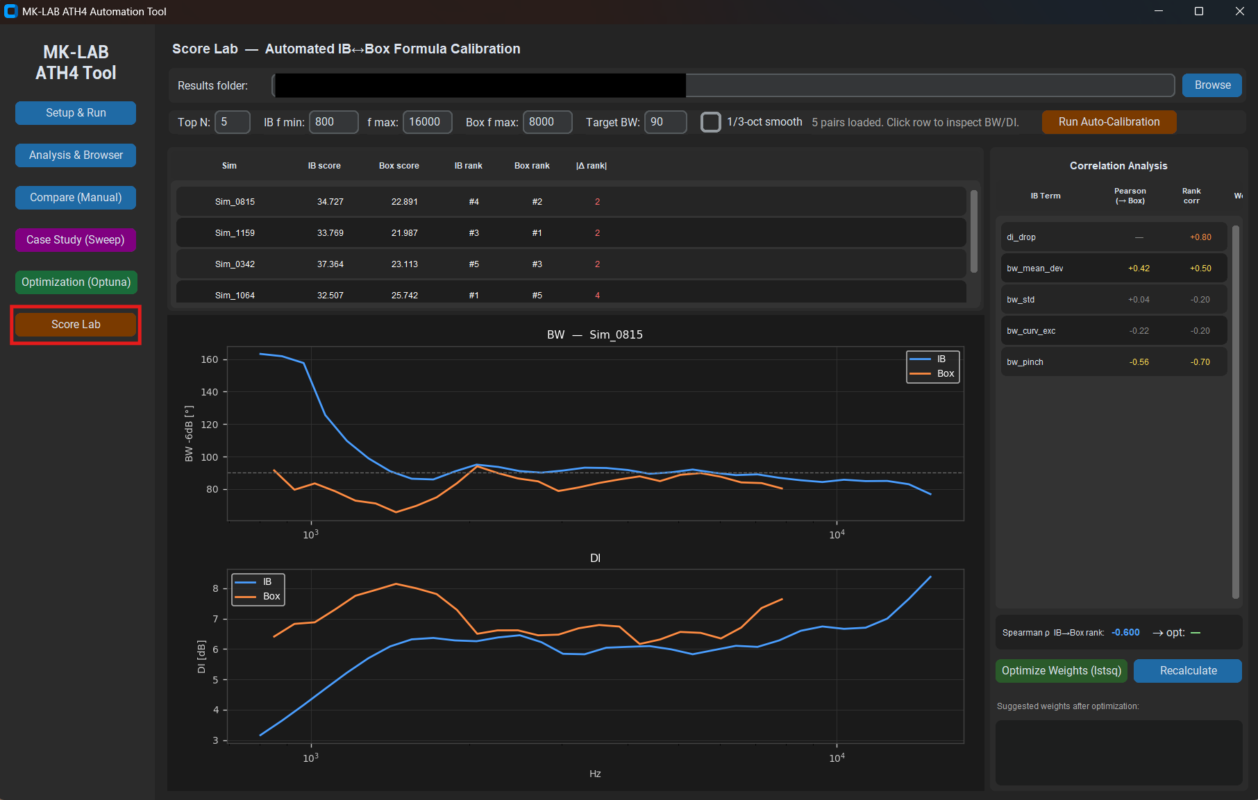
A high rank correlation (ρ > 0.85) means the IB optimiser is reliably selecting designs that translate well to real mounting conditions. A low correlation means the scoring formula is tracking the wrong features — and the per-term Pearson analysis points directly at which terms to retune. This creates a feedback loop: optimise on IB, validate on box, update weights, repeat.
Rank correlation with 5 data points is indicative, not conclusive. For ρ to be statistically significant at p < 0.05 with n = 5, you need |ρ| > 0.88. I treat small-batch Score Lab results as a directional signal — and aim for at least 12–15 pairs before adjusting weights with confidence.
What the Tool Is Not
It is worth being explicit about the limits.
The tool optimises acoustic radiation pattern. It says nothing about the mechanical properties of the waveguide — resonances, material damping, surface finish. A design that scores well in BEM simulation can still fail physically if the geometry is impossible to manufacture or if the throat geometry excites a membrane mode in the compression driver.
It also does not model the driver itself. The throat boundary condition is a uniform-velocity piston — a clean, idealised source. Real compression drivers have non-uniform diaphragm motion, phase plug insertion loss, and a rising distortion floor at high SPL. The simulation is an upper bound on what the waveguide can do, not a prediction of what the complete system will measure.
And the OSSE is a starting model, not a guarantee. The mathematical basis gives ATH4 a strong prior for what a constant-directivity profile should look like, but the acoustic truth is always in the BEM result. The tool takes the OSSE geometry seriously as a starting point and lets simulation decide how far reality deviates from the ideal.
Used correctly — as a fast pre-filter that removes clearly bad geometries so physical prototypes can focus on genuinely competitive candidates — it compresses the development timeline substantially. Used carelessly, it produces confident-looking numbers for designs that were never going to work.